Matlab has many possibilities to create plots even fancy ones. However its defaults are very seldom suitable to use the plots directly for a publication. The following minimal code demonstrates how to generate a pcolor plot for 2D data with x- and y-axis. The data was calculated using the function shown here.
pcolor(xAxis, yAxis, Data2D); shading flat; % do not interpolate pixels colorbar % add colorbar xlabel('x / µm'); ylabel('y / µm'); |
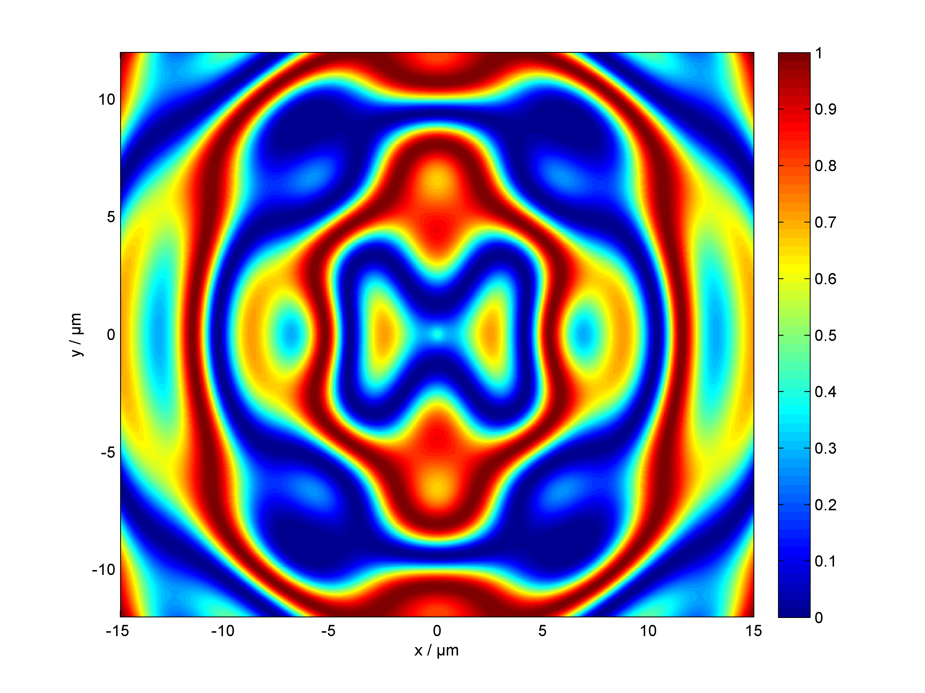
This however is not optimal. Font and fontsizes are not optimal, the color depth should be higher and tics are not shown anymore. Furthermore the colorbar should have an label as well.
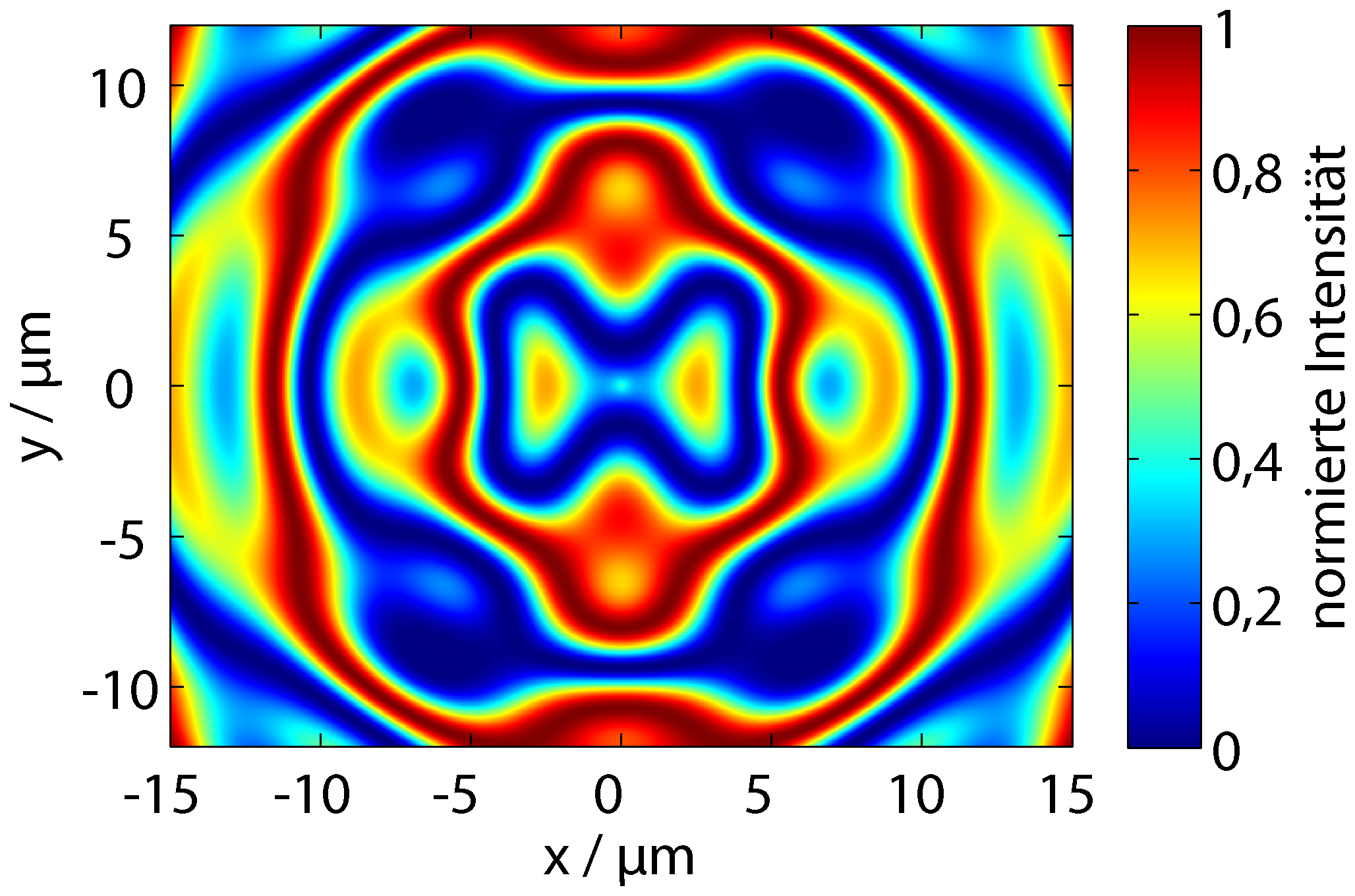
The following code demonstrates a general approach how to solve all these problems and achieve directly a plot output which can be used directly for publications. The followin picture shows the resulting image:
First the environment is set up (not necessary if you just want to plot) and variables for plotting are defined.
% clear command window, figures and all variables clc; clf; clear all; %% Common variables FontSize = 12; FontName = 'MyriadPro-Regular'; % or choose any other font doExportPlot = true; languageEnglish = false; |
Next, the data for plotting is created. Here a previous shown example is used
%% Calculation % calculate in single line (fastest method) xMat = (xAxis' * ones([1 yPoints]))'; yMat = yAxis' * ones([1 xPoints]); Data2D = Ripple(xMat, yMat); Data2D = Data2D - min(min(Data2D)); % normalize to 0-1 Data2D = Data2D / max(max(Data2D)); |
Then the plot window is opened and configured. Here a fixed size in cm is used. The z-buffer is used because opengl has rounding errors and should therefore be avoided if not necessary. Furthermore the position of the plot within the window is configured.
%% start plot % figure dimensions in cm. I choose 1.5 or 2 times % the target size typically. If figure is display in % document much smaller increase the fontsize. figure_width = 14; figure_height = 10; % --- setup plot windows figuresVisible = 'on'; % 'off' for non displayed plots (will still be exported) hfig = figure(1); clf; set(hfig,'Visible', figuresVisible) set(hfig, 'units', 'centimeters', 'pos', [5 5 figure_width figure_height]) set(hfig, 'PaperPositionMode', 'auto'); set(hfig, 'Renderer','Zbuffer'); set(hfig, 'Color', [1 1 1]); % Sets figure background set(gca, 'Color', [1 1 1]); % Sets axes background % --- dimensions and position of plot hsp = subplot(1,1,1, 'Parent', hfig); set(hsp,'Position',[0.15 0.17 0.75 0.80]); |
The actual plot is still a few lines:
%% plot colorDepth = 1000; colormap(jet(colorDepth)); pcolor(xAxis, yAxis, Data2D); |
Now the plot needs to be configured. First the pcolor must not have black lines between each data point (the plot would be black). This is achieved by setting the shading. In case of flat not interpolation is done. This might look nicer, but in case of scientific data is close to cheating. The axis properties are important, because matlab does not care itself about scaling. This means that the x- and y-axis might be square although the axis values have a factor of 1:10. The image ratio is set to the axis ratio by the property ‘image’. Additionally several properties for the figure can be set. Most important are the TickLength and the LineWidth.
%% setup axis plot properties % shading interp; % interpolate pixels shading flat; % do not interpolate pixels axis on; % display axis axis tight; % no white borders axis image; % real x,y scaling set(gca, ... 'CLim' , [0 1], ... 'Box' , 'on' , ... 'TickDir' , 'in' , ... 'TickLength' , [.015 .015] , ... 'XMinorTick' , 'off' , ... 'YMinorTick' , 'off' , ... 'XGrid' , 'off' , ... 'YGrid' , 'off' , ... 'XColor' , [.0 .0 .0], ... 'YColor' , [.0 .0 .0], ... 'LineWidth' , 0.6 ); |
optionally the axis ticks can be configured
%% axis ticks set(gca,'XTick',-15:5:15) set(gca,'YTick',-10:5:10) |
Next the axis labels are set up. Here I define them in both german end english. That has the advantage, that I can create the figure easily in both languages. The labels are all set with saving of handles, to be able to configure them later.
%% label texts TITLE = ''; if (languageEnglish) xLabelText = 'x / µm'; yLabelText = 'y / µm'; zLabelText = 'normalized intensity'; else xLabelText = 'x / µm'; yLabelText = 'y / µm'; zLabelText = 'normierte Intensität'; end % save handles to set up label properties hTitle = title(TITLE); hXLabel = xlabel(xLabelText); hYLabel = ylabel(yLabelText); |
The colorbar is still missing. Here a label and ticks are defined, and the TickLength and LineWidth is configured.
%% colorbar caxis([0 1]); hcb = colorbar('location','EastOutside'); hcLabel = ylabel(hcb,zLabelText); set(hcb,'YTickLabel',0:0.2:1, 'Ytick', 0:0.2:1) set(hcb,'YTickMode','manual') set(hcb, ... 'Box' , 'on' , ... 'TickDir' , 'in' , ... 'TickLength' , [.015 .015] , ... 'LineWidth' , 0.6); |
Last all handles need to be configured. Basically that means setting up the fonts for all.
%% set properties for all handles set([gca, hcb, hTitle, hXLabel, hYLabel, hcLabel], ... 'FontSize' , FontSize , ... 'FontName' , FontName); |
And finally some bugs need to be fixed. fixLabels changes the decimal point character to ‘,’ (see below) and the last line brings the tics to the top again, which are overwritten by matlab.
%% last 'bug' fixes % change decimal point to ',' for german text if (~languageEnglish) fixLabels(gca); fixLabels(hcb); end % bring axis on top again (fix matlab bug) set(gca,'Layer', 'top'); |
function fixLabels( axis )

xlabels = get(axis, 'XTickLabel');
for k=1:size(xlabels,1)
    xlabels(k,:) = strrep(xlabels(k,:), '.', ',');
end
set(axis, 'XTickLabel', xlabels);

ylabels = get(axis, 'YTickLabel');
for k=1:size(ylabels,1)
    ylabels(k,:) = strrep(ylabels(k,:), '.', ',');
end
set(axis, 'YTickLabel', ylabels);

set(axis, 'XTickMode', 'manual');
set(axis, 'YTickMode', 'manual');

end |
In the end we might want to export the plot. Here the printing is done to a png file with a resolution of 400 dpi. Since matlab is not filling the plot window and large white borders might surround the actual plot, the png file is cropped using the crop function by Andrew Bliss.
%% export drawnow SaveDir = ''; SaveName = 'pcolor-example'; if (doExportPlot) IMAGENAME = [SaveDir SaveName]; print(hfig, ['-r' num2str(400)], [IMAGENAME '.png' ], ['-d' 'png']); crop([IMAGENAME '.png']); display('finished plot export') end % close(hfig); |
 PcolorExample.m (4,1 KiB)